
Introduction to Statistics for Nursing Students
Comprehensive guide to understanding statistical concepts and applications in nursing
Table of Contents
1. Definition and Use of Statistics
What is Statistics?
Statistics is a branch of mathematics concerned with collecting, analyzing, interpreting, and presenting data to describe patterns, make predictions, and draw meaningful conclusions.
Why Statistics Matter in Nursing
Clinical Practice
- Interpreting patient vital signs and lab values
- Understanding medication efficacy rates
- Evaluating treatment outcomes
- Monitoring disease prevalence
Research
- Designing nursing research studies
- Analyzing research findings
- Interpreting published research
- Contributing to evidence-based practice
Mnemonic: “CARE”
Collect data that matters
Analyze data accurately
Report findings clearly
Evaluate implications for practice
Example: Statistics in Action
A nurse collects blood pressure readings from 50 patients before and after implementing a new relaxation technique. Using statistical analysis, the nurse can determine if the technique significantly reduces blood pressure and make evidence-based recommendations for practice.
2. Scales of Measurement
In statistics, data is classified into four measurement scales, each with different properties and appropriate statistical methods.
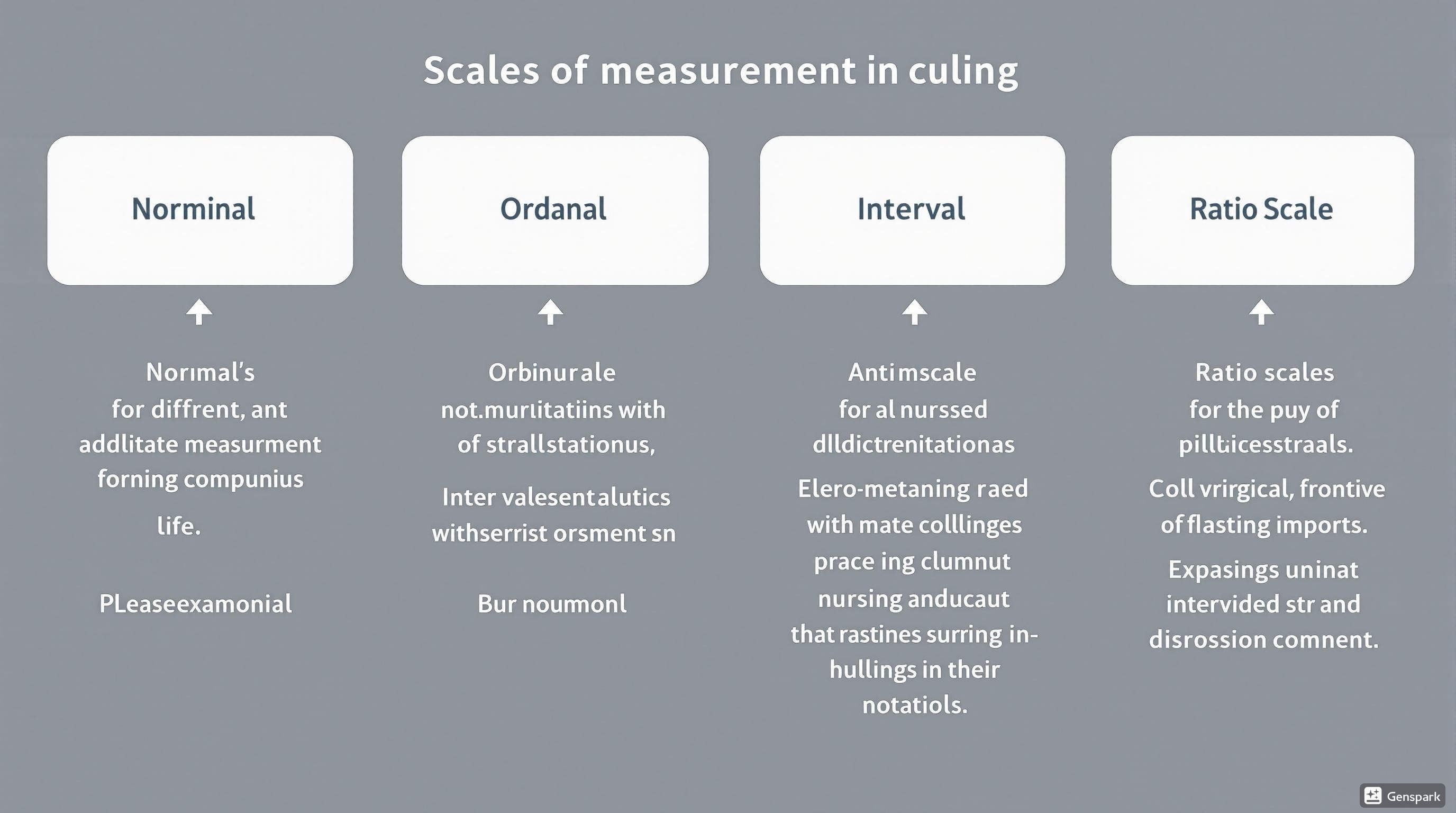
Nominal Scale
Definition: Categorizes data without any order or ranking.
Properties: Categories are mutually exclusive with no numerical significance.
Nursing Examples:
- Gender (male/female)
- Blood type (A, B, AB, O)
- Diagnosis codes
- Hospital unit categories
Appropriate Statistics: Mode, frequency counts, percentages, chi-square test
Ordinal Scale
Definition: Categories with a clear order or ranking, but without equal intervals.
Properties: Ordered categories, but differences between values aren’t consistent.
Nursing Examples:
- Pain scales (0-10)
- Pressure ulcer staging (I-IV)
- Likert scales (strongly disagree to strongly agree)
- Triage categories (emergent, urgent, non-urgent)
Appropriate Statistics: Median, mode, percentiles, Spearman correlation
Interval Scale
Definition: Ordered values with equal intervals but no true zero point.
Properties: Equal spacing between values, but ratios aren’t meaningful.
Nursing Examples:
- Temperature in Celsius or Fahrenheit
- Calendar dates
- IQ scores
- Some mental health assessment scores
Appropriate Statistics: Mean, median, mode, standard deviation, Pearson correlation
Ratio Scale
Definition: Ordered values with equal intervals and a true zero point.
Properties: Highest level of measurement; ratios are meaningful.
Nursing Examples:
- Blood pressure readings
- Weight, height
- Lab values (hemoglobin, glucose)
- Time measurements (length of hospital stay)
Appropriate Statistics: All statistical measures, including geometric mean and coefficient of variation
Mnemonic: “NOIR”
Nominal (Names) – Categories without order
Ordinal (Order) – Ranked but unequal intervals
Interval (Intervals) – Equal gaps, no true zero
Ratio (Ratios) – Equal gaps with true zero
Example: Identifying Measurement Scales
A nurse researcher is studying patient recovery after surgery and collects the following data:
- Nominal: Surgical procedure type (appendectomy, cholecystectomy, etc.)
- Ordinal: Post-operative pain levels (mild, moderate, severe)
- Interval: Patient satisfaction score (1-5 scale)
- Ratio: Length of hospital stay in days
Understanding these scales helps the researcher select appropriate statistical tests for analysis.
3. Frequency Distribution and Graphical Presentation
What is a Frequency Distribution?
A frequency distribution is an organized tabulation of individual data values showing the frequency (count) or percentage of observations in each data category or interval.
Types of Frequency Distributions
Simple Frequency Distribution
Shows the number of occurrences for each data value.
Example: Blood Types of 50 Patients
| Blood Type | Frequency |
|---|---|
| A | 20 |
| B | 12 |
| AB | 5 |
| O | 13 |
Relative Frequency Distribution
Shows the percentage of occurrences for each value.
Example: Blood Types of 50 Patients
| Blood Type | Frequency | Relative Frequency |
|---|---|---|
| A | 20 | 40% |
| B | 12 | 24% |
| AB | 5 | 10% |
| O | 13 | 26% |
Cumulative Frequency Distribution
Shows the accumulation of frequencies up to each data value.
Example: Patient Ages in Hospital Ward
| Age Group | Frequency | Cumulative Frequency |
|---|---|---|
| 18-30 | 8 | 8 |
| 31-45 | 12 | 20 |
| 46-60 | 15 | 35 |
| 61-75 | 10 | 45 |
| 76-90 | 5 | 50 |
Grouped Frequency Distribution
Groups continuous data into intervals or classes.
Example: Systolic Blood Pressure Readings
| Blood Pressure (mmHg) | Frequency |
|---|---|
| 90-109 | 5 |
| 110-129 | 18 |
| 130-149 | 14 |
| 150-169 | 8 |
| 170-189 | 5 |
Graphical Presentation of Data
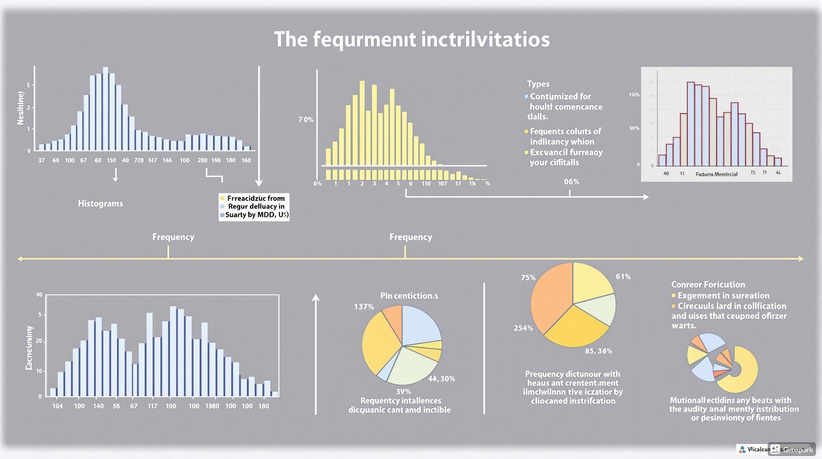
Bar Graph
Best for: Categorical (nominal and ordinal) data
Nursing Applications:
- Comparing patient demographics
- Displaying medication frequencies
- Showing disease incidence by department
Histogram
Best for: Continuous (interval and ratio) data
Nursing Applications:
- Displaying distribution of patient ages
- Showing distribution of lab values
- Analyzing length of hospital stays
Pie Chart
Best for: Showing proportions of a whole
Nursing Applications:
- Allocation of nursing time to different tasks
- Distribution of patient diagnoses
- Budget allocation in healthcare facilities
Line Graph
Best for: Showing trends over time
Nursing Applications:
- Tracking vital signs over time
- Monitoring infection rates
- Following patient improvement during treatment
Box Plot
Best for: Showing distribution and identifying outliers
Nursing Applications:
- Comparing lab values between patient groups
- Analyzing pain scores across treatments
- Studying distribution of hospital readmission times
Scatter Plot
Best for: Showing relationships between two variables
Nursing Applications:
- Examining relationship between BMI and blood pressure
- Studying correlation between stress and sleep quality
- Analyzing association between age and recovery time
Mnemonic: “GRAPHS”
Group data meaningfully
Represent visually with suitable charts
Analyze patterns and trends
Present findings clearly
Highlight key insights
Support with appropriate statistics
Example: Choosing the Right Graph
A nurse manager wants to analyze data about pressure ulcer incidence in different hospital units:
- Bar graph: To compare pressure ulcer rates between different units
- Pie chart: To show distribution of pressure ulcer stages
- Line graph: To track pressure ulcer rates over the past 12 months
- Scatter plot: To examine relationship between length of stay and pressure ulcer development
Each graph type reveals different insights from the same dataset.
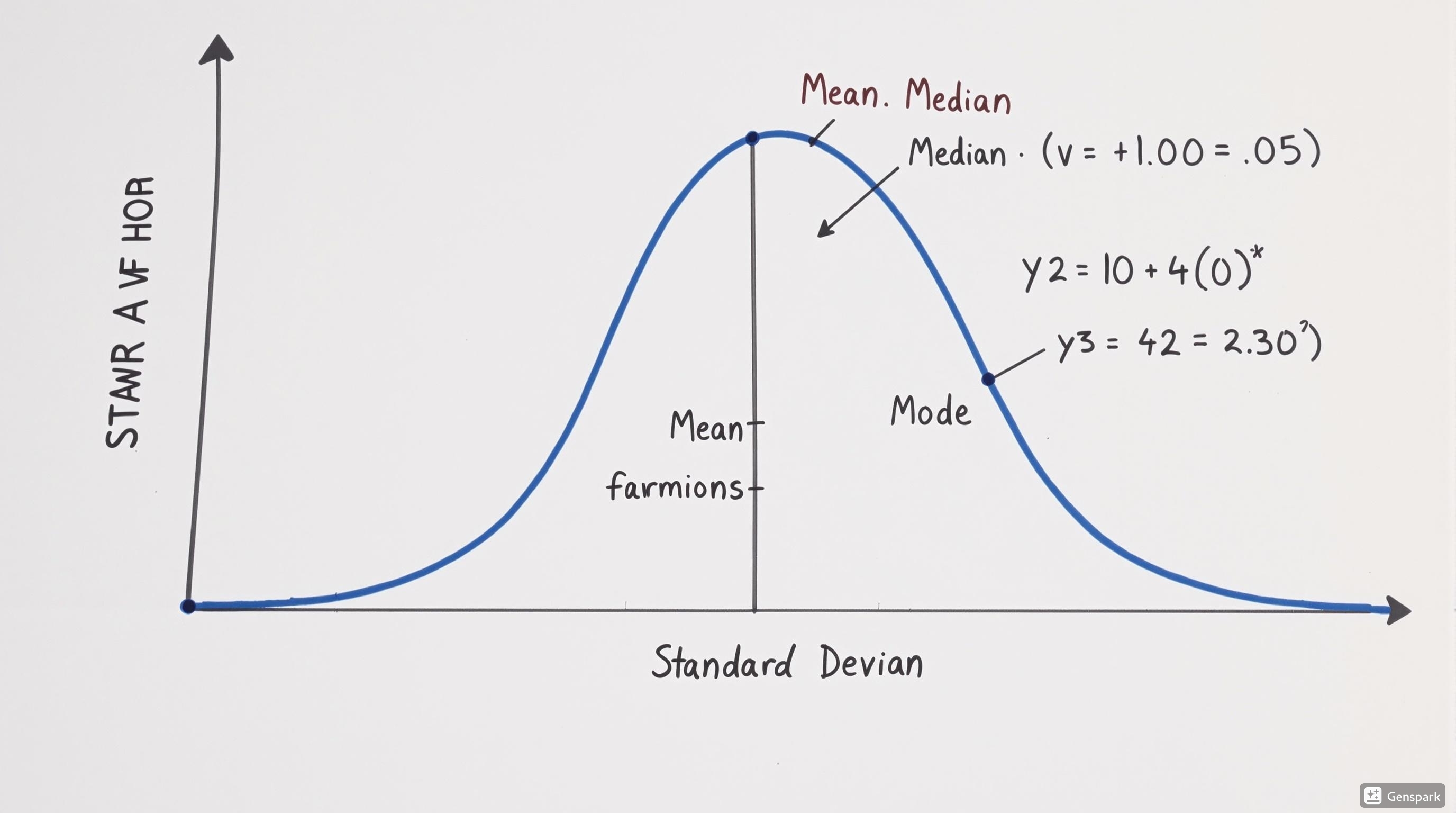
4. Mean, Median, Mode, and Standard Deviation
Measures of Central Tendency
Measures of central tendency describe the center or typical value of a dataset. The three main measures are mean, median, and mode.
Mean
Definition: The arithmetic average of all values.
Where:
- Σx = sum of all values
- n = number of values
Best used when: Data is normally distributed without extreme outliers.
Nursing Example: Average heart rate of patients in a unit.
Median
Definition: The middle value when data is arranged in order.
How to find:
- Arrange data in ascending order
- If n is odd, median is the middle value
- If n is even, median is average of two middle values
Best used when: Data has outliers or is skewed.
Nursing Example: Median length of hospital stay.
Mode
Definition: The most frequently occurring value(s).
Properties:
- Data can have one mode (unimodal)
- Data can have two modes (bimodal)
- Data can have more than two modes (multimodal)
- Data can have no mode
Best used when: Identifying the most common category or value.
Nursing Example: Most common chief complaint in ER.
Example: Calculating Mean, Median, and Mode
A nurse collected systolic blood pressure readings (mmHg) from 9 patients:
118, 124, 136, 128, 142, 118, 132, 145, 128
Mean:
Sum = 118 + 124 + 136 + 128 + 142 + 118 + 132 + 145 + 128 = 1171
Mean = 1171 ÷ 9 = 130.1 mmHg
Median:
Ordered: 118, 118, 124, 128, 128, 132, 136, 142, 145
Median = 128 mmHg (5th value)
Mode:
118 appears twice
128 appears twice
Mode = 118 and 128 mmHg (bimodal)
Measure of Dispersion: Standard Deviation
Standard Deviation
Standard deviation (SD) measures how spread out the values in a dataset are from the mean. It indicates the typical distance between each data point and the mean.
Standard Deviation (σ) = √[(Σ(x – x̄)²) / n]
Where:
- x = each individual value
- x̄ = mean of all values
- n = number of values
- Σ = sum of
Interpreting Standard Deviation
- Small SD: Data points are close to the mean (less variability)
- Large SD: Data points are spread out from the mean (more variability)
- In a normal distribution:
- 68% of data falls within ±1 SD of the mean
- 95% of data falls within ±2 SD of the mean
- 99.7% of data falls within ±3 SD of the mean
Nursing Applications
- Understanding lab reference ranges (typically mean ±2 SD)
- Identifying abnormal vital signs
- Comparing variability between patient groups
- Evaluating consistency of clinical measurements
- Interpreting research findings
Example: Standard Deviation in Practice
A hospital unit measures the time (in minutes) it takes to administer medications to patients:
8, 12, 9, 15, 10
Step 1: Calculate the mean
Mean = (8 + 12 + 9 + 15 + 10) ÷ 5 = 54 ÷ 5 = 10.8 minutes
Step 2: Calculate deviations from the mean and square them
| Value (x) | Deviation (x – x̄) | (x – x̄)² |
|---|---|---|
| 8 | 8 – 10.8 = -2.8 | 7.84 |
| 12 | 12 – 10.8 = 1.2 | 1.44 |
| 9 | 9 – 10.8 = -1.8 | 3.24 |
| 15 | 15 – 10.8 = 4.2 | 17.64 |
| 10 | 10 – 10.8 = -0.8 | 0.64 |
| Sum of squared deviations: | 30.8 | |
Step 3: Calculate standard deviation
SD = √(30.8 ÷ 5) = √6.16 = 2.48 minutes
This means that the medication administration times typically vary by about ±2.48 minutes from the mean time of 10.8 minutes.
Mnemonic: “MMM-SD”
Mean for normal distributions without outliers
Median for skewed data or when outliers present
Mode for most common category
Standard Deviation for understanding variation
5. Normal Probability and Tests of Significance
Normal Probability Distribution
The normal distribution (also called Gaussian or bell curve) is a continuous probability distribution that is symmetrical around its mean. Many biological and health measurements follow this distribution.
Properties of the Normal Distribution
Key Characteristics
- Bell-shaped and symmetrical around the mean
- Mean, median, and mode are all equal
- Defined by two parameters: mean (μ) and standard deviation (σ)
- Total area under the curve equals 1 (100% probability)
- Extends infinitely in both directions but approaches zero
The 68-95-99.7 Rule
- 68% of data falls within ±1 SD of the mean
- 95% of data falls within ±2 SD of the mean
- 99.7% of data falls within ±3 SD of the mean
This rule is essential for interpreting lab values, vital signs, and other health measurements.
Example: Normal Distribution in Nursing
Hemoglobin levels in adult women approximately follow a normal distribution with a mean (μ) of 14 g/dL and a standard deviation (σ) of 1 g/dL. Using the 68-95-99.7 rule:
- 68% of women have hemoglobin between 13-15 g/dL (14 ± 1)
- 95% of women have hemoglobin between 12-16 g/dL (14 ± 2)
- 99.7% of women have hemoglobin between 11-17 g/dL (14 ± 3)
Values outside the 95% range (below 12 or above 16) might be considered clinically significant and warrant further investigation.
Tests of Significance
Hypothesis Testing and Statistical Significance
Statistical significance testing helps determine whether observed results are likely due to chance or represent a real effect. This process involves formulating and testing hypotheses.
Hypothesis Testing Process
- State hypotheses:
- Null hypothesis (H₀): No effect or relationship
- Alternative hypothesis (H₁): An effect or relationship exists
- Set significance level: Usually α = 0.05
- Select appropriate test: Based on data type and research question
- Calculate test statistic and p-value
- Make decision: Reject or fail to reject null hypothesis
- Interpret results: Clinical significance vs. statistical significance
Common Statistical Tests
| Test | When to Use |
|---|---|
| t-test | Compare means of two groups |
| ANOVA | Compare means of three or more groups |
| Chi-square | Compare proportions/categorical data |
| Pearson’s r | Measure linear correlation |
| Mann-Whitney U | Compare two groups (non-parametric) |
| Wilcoxon | Compare paired observations (non-parametric) |
P-value Interpretation
A p-value is the probability of observing results at least as extreme as the current results if the null hypothesis were true.
- p < 0.05: Results are statistically significant; reject null hypothesis
- p ≥ 0.05: Results are not statistically significant; fail to reject null hypothesis
Important: Statistical significance does not always equal clinical significance. A statistically significant result may have little practical importance in patient care.
Example: Hypothesis Testing in Nursing Research
A nurse researcher wants to test if a new pain management protocol reduces post-operative pain scores compared to standard care.
- H₀: No difference in pain scores between new protocol and standard care
- H₁: New protocol results in lower pain scores than standard care
- Test: Independent samples t-test
- Results: Mean pain score (standard care) = 6.8, Mean pain score (new protocol) = 5.3, p = 0.028
- Conclusion: Since p < 0.05, the researcher rejects the null hypothesis and concludes that the new protocol significantly reduces pain scores compared to standard care.
- Clinical significance: A reduction of 1.5 points on a 10-point pain scale may be clinically meaningful for patients and influence practice.
Mnemonic: “NURSE”
Null hypothesis statement
Understand what test to use
Run statistical analysis
Significant or not? Check p-value
Evaluate clinical importance
6. Coefficient of Correlation
What is Correlation?
Correlation measures the strength and direction of the linear relationship between two variables. The correlation coefficient (r) quantifies this relationship.
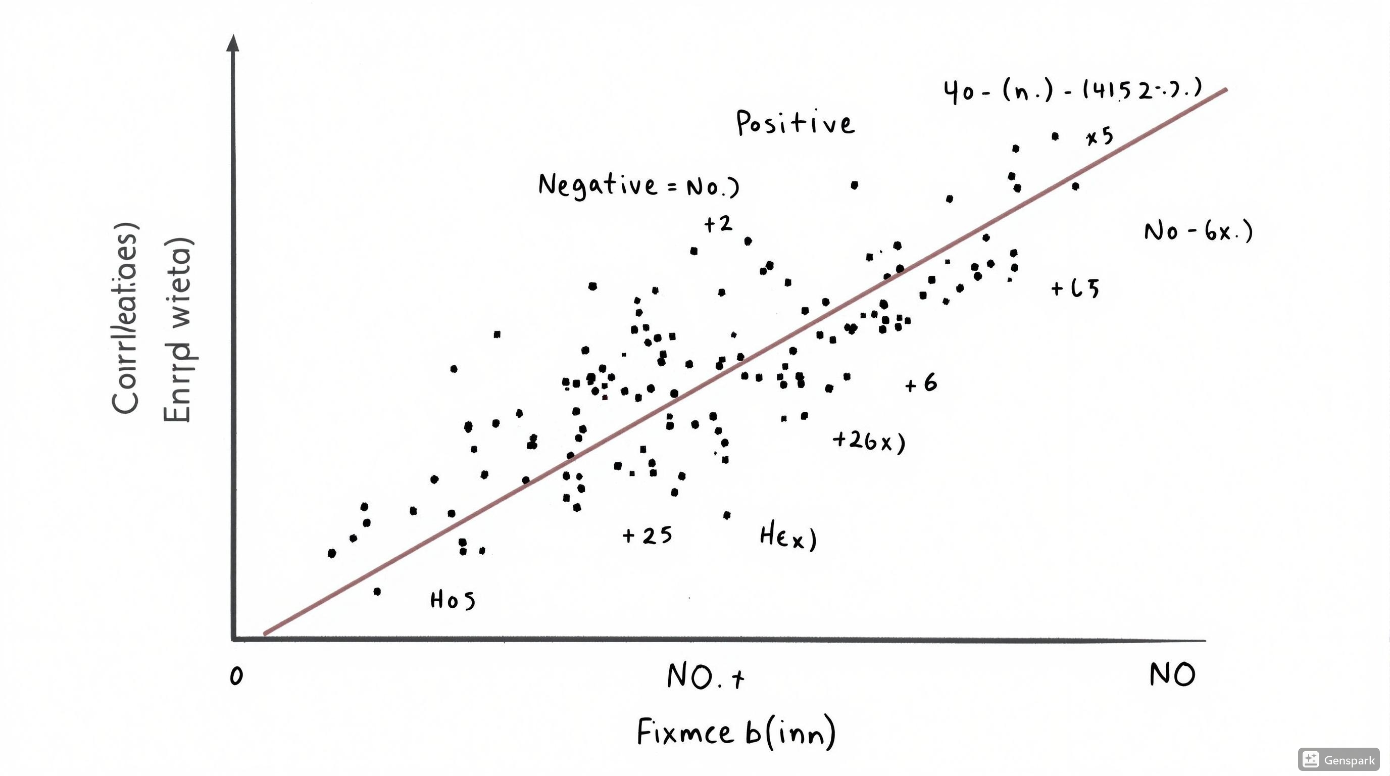
Properties of Correlation Coefficient
Key Characteristics
- Values range from -1 to +1
- +1 indicates perfect positive correlation
- -1 indicates perfect negative correlation
- 0 indicates no linear correlation
- Correlation does not imply causation
- Measures only linear relationships
Interpreting Correlation Strength
| Correlation Value | Interpretation |
|---|---|
| 0.00 – 0.19 | Very weak |
| 0.20 – 0.39 | Weak |
| 0.40 – 0.59 | Moderate |
| 0.60 – 0.79 | Strong |
| 0.80 – 1.00 | Very strong |
Note: Same scale applies to negative values.
Types of Correlation Coefficients
Pearson’s Correlation Coefficient (r)
- Measures linear relationship between two continuous variables
- Assumes normal distribution and linear relationship
- Formula:
r = Σ[(x – x̄)(y – ȳ)] / √[Σ(x – x̄)² Σ(y – ȳ)²]
- Nursing Example: Correlation between BMI and blood pressure
Spearman’s Rank Correlation (rho)
- Non-parametric alternative to Pearson’s
- Used when data is ordinal or does not meet assumptions for Pearson’s
- Measures monotonic relationships (when variables tend to change together, but not necessarily at a constant rate)
- Nursing Example: Correlation between pain scale ratings and medication dosage
Example: Correlation in Nursing Research
A nurse researcher collected data on hours of sleep (x) and anxiety scores (y) from 10 patients:
| Patient | Hours of Sleep (x) | Anxiety Score (y) |
|---|---|---|
| 1 | 4 | 9 |
| 2 | 5 | 7 |
| 3 | 6 | 6 |
| 4 | 7 | 5 |
| 5 | 8 | 4 |
| 6 | 3 | 10 |
| 7 | 9 | 3 |
| 8 | 5 | 8 |
| 9 | 7 | 4 |
| 10 | 6 | 5 |
Calculating Pearson’s correlation coefficient gives r = -0.94
Interpretation:
- The negative sign indicates an inverse relationship: as hours of sleep increase, anxiety scores decrease
- The magnitude (0.94) indicates a very strong correlation
- This suggests that sleep and anxiety are strongly related in this patient group
- Note: This doesn’t prove that lack of sleep causes anxiety or vice versa (correlation ≠ causation)
Important Considerations
- Correlation does not imply causation: Two variables may be correlated because they are both influenced by a third variable
- Outliers can significantly affect correlation: Always visualize data with a scatter plot
- Correlation only measures linear relationships: Two variables may have a strong non-linear relationship even if r is close to 0
- Sample size matters: Correlations from small samples may not be reliable
Mnemonic: “CORDS”
Correlation value (-1 to +1)
Observe the direction (positive or negative)
Review the strength (weak, moderate, strong)
Don’t assume causation
Scatter plot to visualize
7. Statistical Packages and Applications
Statistical Software in Nursing Research
Statistical packages are specialized software designed to perform statistical analyses efficiently and accurately. These tools are essential for managing and analyzing data in nursing research.
Common Statistical Packages
SPSS
Statistical Package for the Social Sciences
- Most widely used in nursing research
- User-friendly point-and-click interface
- Comprehensive statistical capabilities
- Excellent for survey data analysis
- Powerful data visualization tools
R
Open-source Statistical Software
- Free and open-source
- Highly flexible with extensive packages
- Superior graphics capabilities
- Powerful for advanced statistical methods
- Steeper learning curve (programming-based)
SAS
Statistical Analysis System
- Enterprise-level statistics software
- Excellent for large datasets
- Highly reliable and validated
- Comprehensive data management tools
- Common in healthcare organizations
Microsoft Excel
Spreadsheet with Statistical Functions
- Widely available and accessible
- Good for basic statistics
- Suitable for small datasets
- Built-in data visualization tools
- Limited advanced statistical capabilities
Stata
Integrated Statistical Software
- Balance of usability and power
- Strong in epidemiological research
- Excellent documentation
- Good data management capabilities
- Popular in healthcare research
EpiInfo
CDC-developed Software
- Free software from CDC
- Designed for epidemiology research
- Easy to learn and use
- Good for survey and questionnaire design
- Limited advanced statistics
Applications in Nursing
Research Applications
- Analyzing clinical trial data
- Processing survey responses
- Determining intervention effectiveness
- Exploring relationships between variables
- Testing nursing theories
- Meta-analysis of existing research
Clinical Applications
- Quality improvement initiatives
- Patient outcome tracking
- Performance monitoring
- Resource utilization analysis
- Risk assessment modeling
- Decision support systems
Example: Statistical Software in Action
A nurse researcher is studying the impact of a new discharge education protocol on readmission rates for heart failure patients.
Research Process:
- Data collection from medical records
- Entering data into SPSS
- Data cleaning and validation
- Descriptive statistics generation
- Comparative analysis (t-test)
- Creating visualization for findings
- Interpreting and reporting results
Statistical Tools Used:
- SPSS for primary analysis
- Excel for initial data management
- Descriptive statistics: mean, median, standard deviation
- Inferential statistics: independent samples t-test
- Kaplan-Meier survival curve for readmission timing
- Bar graphs and line charts for visual presentation
Tips for Choosing Statistical Software
- Consider your needs: Research goals, sample size, complexity of analysis
- Evaluate your skills: Some programs require more statistical and technical knowledge
- Check availability: Many institutions provide licenses for specific software
- Assess support resources: Training, documentation, and community help
- Consider future needs: Software that can grow with your research skills
Mnemonic: “STATS”
Select appropriate software for your needs
Train yourself properly before analysis
Analyze data with the right statistical tests
Thoroughly document your process
Share results with clear visualizations